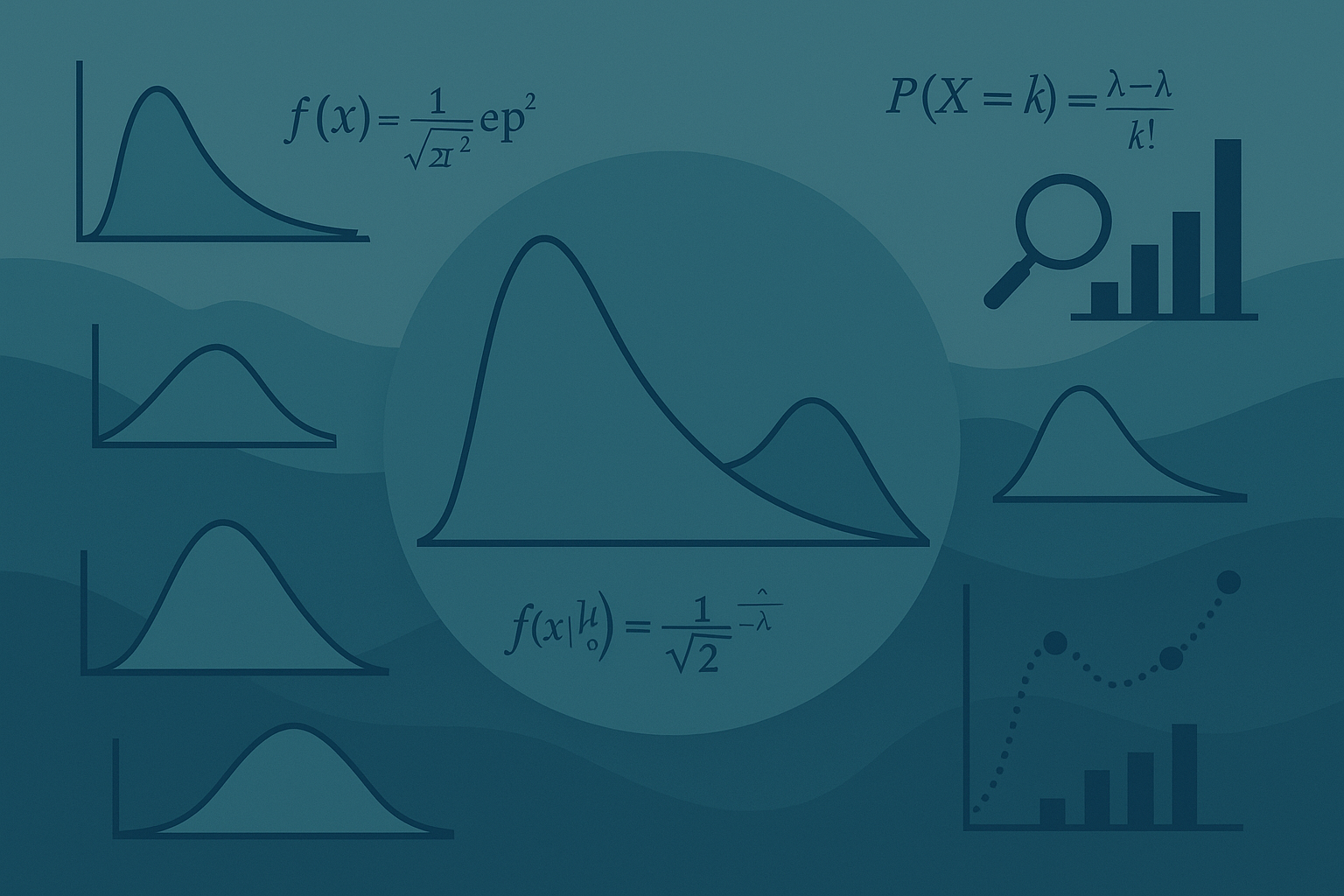
A strategic decision is a large, consequential bet on the future. What makes this difficult, of course, is that you can't actually predict the future. The best you can do is list the possible futures that might unfold, assign some likelihood to each, and see what the overall picture looks like. That's what a probability distribution does — it organizes possibilities, quantifies the uncertainty around them, and turns the abstract idea of "risk" into something you can see and reason about.
So, if you are a decision maker, you need to know how to use probability distributions — not construct them, just use them. Constructing probability distributions requires the mathematical rigor that brings back bad memories from your boring statistics classes. Using them, though, just requires some basic knowledge about how they are designed and how to get information out of them.
In fact, you probably already do use them. Every time you have made a decision based on a 'best case', 'worst case', and 'most likely case' scenario, you have used a probability distribution. You've tried to deal with uncertainty by recognizing that there are multiple possible futures. And, you have attempted to describe those futures quantitatively.
The formal "statistics class" distributions just provide for many more possible futures and then take the extra step of telling you how much more likely one future is than another. But, most importantly, they provide a way to see uncertainty and have a conversation about it.
So here is what you need to know…
How do probability distributions work?
A probability distribution is simply a formula. Like any other formula, if you know the variables, you can plug a number into it and get a result.
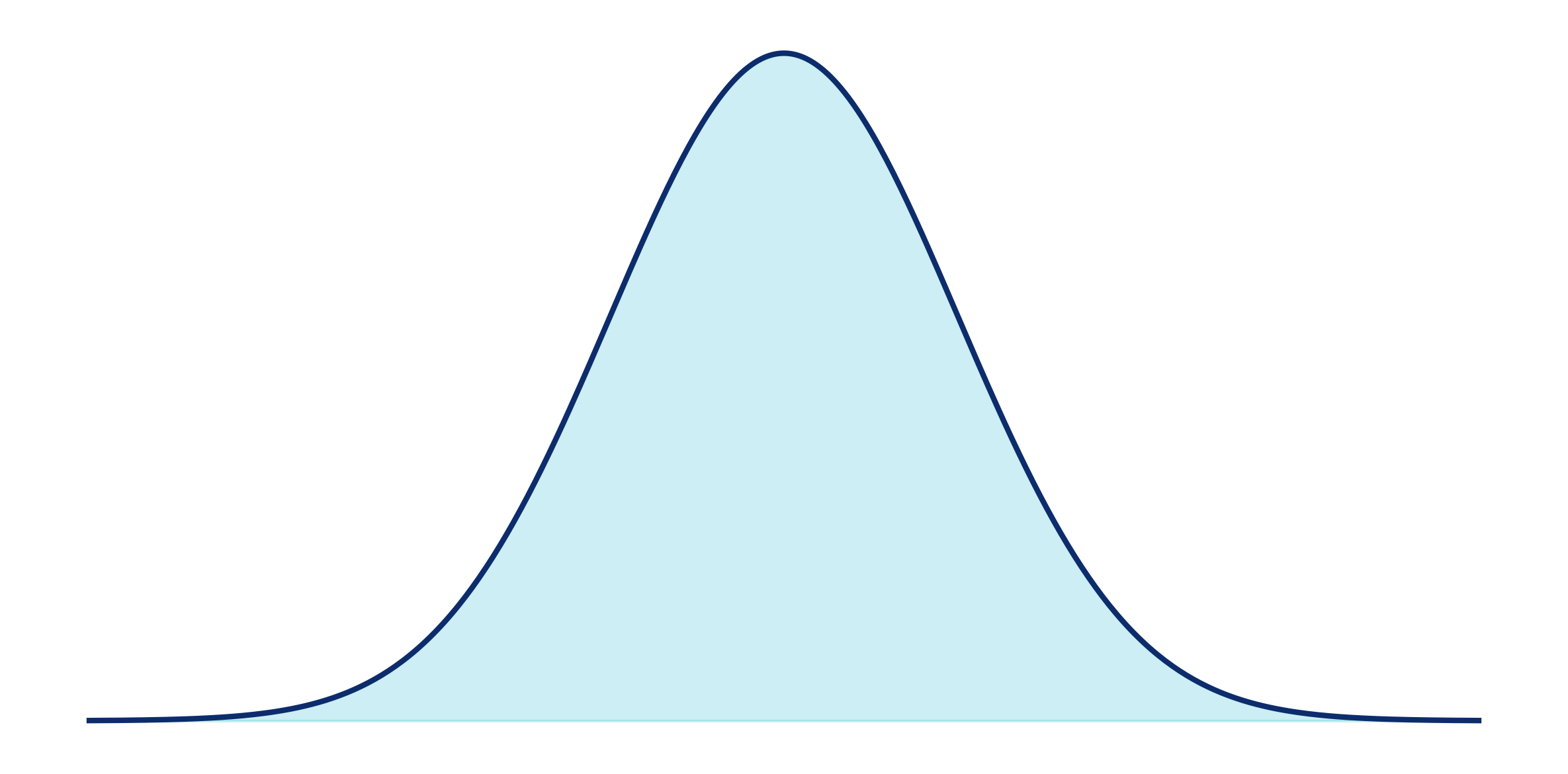
In the case of the Normal distribution (often called the bell curve), the formula looks like this:
f(x∣μ,σ) = 1/√(2πσ²) · exp(−(x−μ)² / (2σ²))
It looks complicated but all it says is that if you know the mean (μ) and the standard deviation (σ) of a variable, you can plug in any number (x) and it will spit out another number. So, let's say that we know that μ = 10 and σ = 2. Then, if we input 5 for the value of x the formula produces approximately 0.009. If x = 10, the formula produces a value of around 0.199.
Because it is called a probability distribution, you might expect that .009 and .199 would be the probability of seeing x. And, for discrete distributions — meaning those where x is a specific, countable outcome like the number of deals closed or customers acquired — you'd be right. The formula would return the probability of that outcome occurring. For most of the distributions you'll use for decisions, though, x can take on any value with any number of decimal places — think of revenue growth rates or market share. The formula that you would use in these cases would be a continuous probability distribution, and the output for each x would be a probability density.
The difference is that probability densities tell you which values are most likely rather than the exact probabilities of those values. It would be like a map that tells you what parts of the ocean are deepest without telling you exactly how deep. Densities are used because the exact probabilities of specific values (x) are essentially 0. The probability of market growth being exactly 2.7% is basically zero because you'd have to exclude 2.7000001%, 2.6999999%, and an infinite number of nearby values.
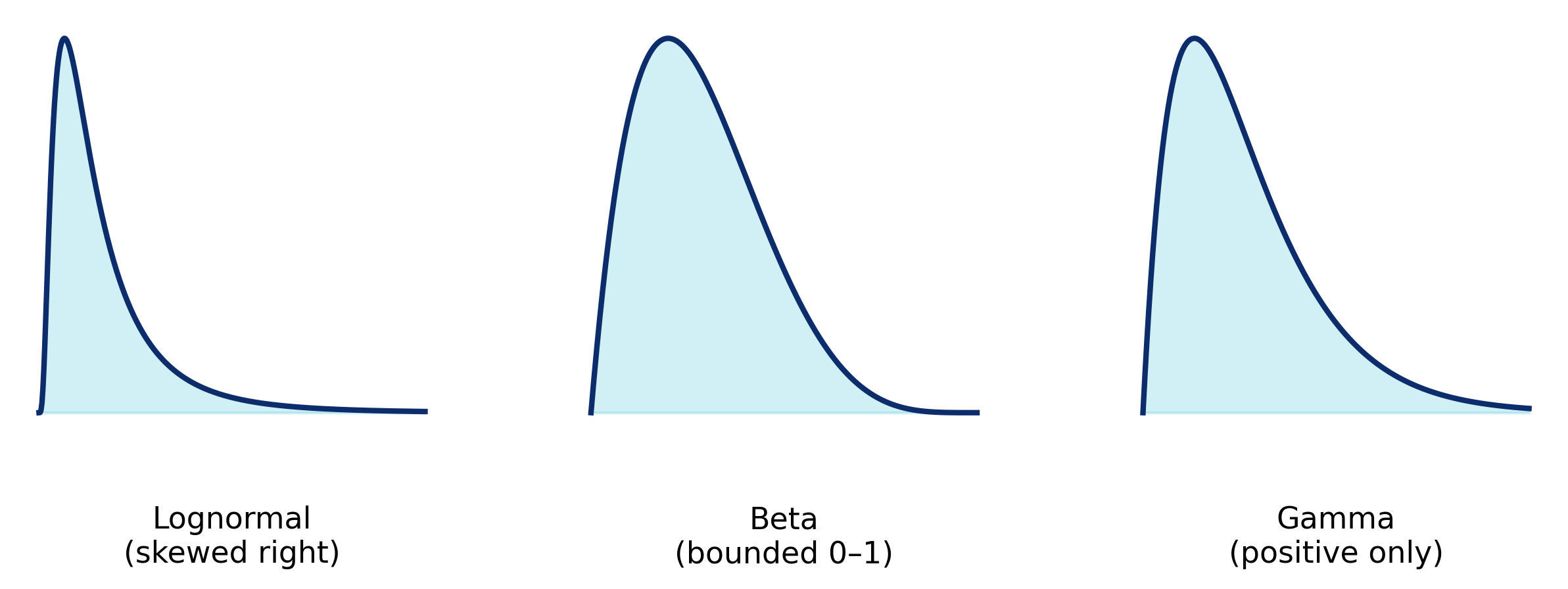
The Normal curve above is actually an example of a continuous distribution so .009 and .199 are densities. However, many more types of distributions exist — both continuous and discrete. And, in practice, the Normal curve often isn't the most useful for business situations. It's used when outcomes are expected to be symmetrical and evenly spread — a pretty rare condition in the business world. Business outcomes tend to be skewed, bounded, or event-driven. So, you're more likely to see distributions like the Lognormal, Beta, or Gamma. They may have different formulas that produce different results for x, but they all serve the same purpose: they describe how likely different outcomes are to occur.
How are they shown?
A big set of probability densities isn't very useful by itself, so they're usually shown in chart form — most often as a smooth curve. Each segment of the curve represents how likely outcomes are to fall within a given range.
Along with the chart, analysts will often offer a bunch of other descriptive statistics such as p-values, confidence intervals, standard error, and so on. Whether or not these are useful depends on what data was used to create the distribution and what question it was meant to answer in the first place.
P-values, etc. tell you how well a sample reflected the population it came from. For example, they can describe how well 1,000 customer surveys represented the attitude of your overall customer base.
Notice that I use the past tense. That is because those statistics tell you how confident you should be in a set of data. And data only gives you a picture of the past.
If you are using a probability distribution to help make strategic decisions, then that distribution should provide a view of possible futures. The inputs will come from models that (hopefully) combine historical data, current trends, causal logic, and expert judgment. So, rather than asking "How well does my data represent reality?" you will need some measure of "How confident can I be that the model represents the future?"
The most commonly used measures of model confidence are credible intervals and sensitivity analysis. Unlike p-values and standard error, though, these are not single statistics you can pull from a spreadsheet or modeling package — they're methods for exploring a model's uncertainty. Because they're not automatic outputs, analysts won't always know to include them. They require running the model multiple times, examining the range of plausible outcomes, and observing changes in results as assumptions shift. In other words, they take judgment and computation, not just syntax. The point is that you might have to ask for this work to be done and it will probably require your strategic input.
How can they be used to make decisions?
When the outputs of a probability distribution are shown in chart form, the x-axis will usually show the futures produced by the model. The y-axis will show their relative likelihood. But, remember that in continuous distributions, the y-axis is not the probability of occurrence, it is the probability density.
In this case, to get actual probabilities, you will need to calculate the area under the curve. For example, if after looking at the chart you think your best case scenario is market growth of more than 2%, you can find the probability of that occurring by calculating the area under the curve for all futures greater than 2%. The same applies for calculating probabilities of growth being between two percentages. Technically, this calculation is accomplished by taking the integral of the probability density in the region of interest. But, don't worry if your calculus is rusty. A computer handles that part in milliseconds. What matters is knowing to ask for probabilities over intervals instead of specific values. This usually comes naturally since what most often matters in decision making are ranges and thresholds.

Of course, as we mentioned above, knowing probabilities is useless unless you also know how confident you should be in them. While neither credible intervals nor scenario analysis directly tell you the degree of confidence you should expect from a model, used together they can show how much trust to place in its predictions.
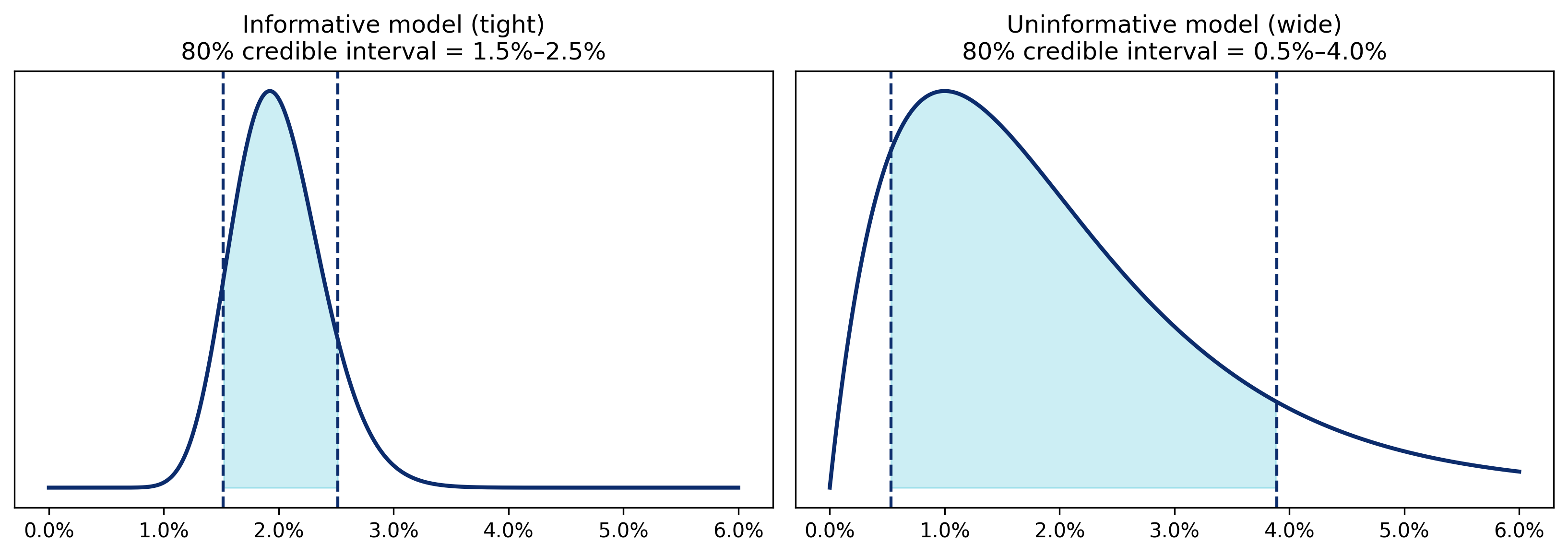
Credible intervals show how valuable or informative a model is. If you ask for the 80% credible interval, you will receive two values — a low and a high value that you can be 80% confident that the true value lies between. The tighter the range, the more credible, or precise, the model might be. So, if in the below market growth model the 80% credible interval lies between 1.5% and 2.5%, we would think that the model is highly informative. But, if the interval is between 0.5% and 4.0%, then the model doesn't really tell you anything you didn't already know, and it is time to rethink the structure and assumptions that went into it.
The problem with this is that in some situations a 1% spread might be excellent. In others, it might be useless. That's why probability distributions are shown as charts — they let you see how uncertainty is shaped and decide whether the credible interval is narrow enough to be useful.
Of course, the model could be precise even with inaccurate assumptions. That's why it's important to also test how much your results depend on the inputs.
Scenario analysis lets you test the model's assumptions by asking, "What happens to the forecast if the model inputs change?" It's like a stress test for your future, and it is fairly simple to perform. You adjust one or more key inputs at a time and see how the shape of the distribution changes — also a reason that distributions are presented visually.
If small changes in assumptions cause large changes in outcomes, you know the model is sensitive and that its predictions are fragile. It is another sign that you need to revisit its structure or improve the quality of its inputs before you can rely on what it's telling you. Scenario analysis and credible intervals complement each other in that credible intervals show how precise the model is, while scenario analysis shows how resilient it is. For example, wide credible intervals but low sensitivity mean the model isn't very precise, but it is stable. You might be able to use its outputs for direction but not for much else.
Narrow intervals but high sensitivity may make the model look confident, but its outputs are not particularly trustworthy. It would be like listening to a meteorologist who swings between clear skies and rain every few minutes — but with a lot of conviction. Ideally, you want a model that's both confident and stable. Or, if that's unachievable, you at least want to know which kind of uncertainty you're managing.
What's the point again?
The point of all this is that probability distributions are more than mathematical constructs learned in statistics classes. They help make the predictions that decisions are built on. They let you visualize and compare multiple possible futures as a landscape of likelihoods. Distributions help you understand the probabilities behind possibilities and make better decisions — if you know how to use them.
← Back to Writing